Knife-Edge Equilibrium

A condition in which something must either be at a precise equilibrium, or else tumble way into catastrophe. In some cases, such as something that really is balanced on a knife's edge, it's an accurate description. However, in models of (say) economic growth, it's a severe flaw in the model.

One of the most famous examples of the knife's edge equilibrium is in the Harrod-Domar Growth Model (1949), which sought to integrate some theory of economic growth with the Keynesian General Theory. Under the Harrod-Domar model, there is a precise rate of investment which is compatible with full employment.

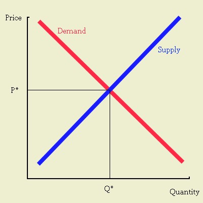
Recall, from Keynes, that investment is one of the determinants of aggregate demand and that aggregate demand is linked to output (or aggregate supply) via the multiplier. Abstracting from all other components, we can write that, in goods market equilibrium:
Y = (1/s)I

where Y is income, I investment, s the marginal propensity to save (and thus the multiplier is 1/s). But investment, note Harrod and Domar, increases the productive capacity of an economy and that itself should change goods market equilbrium.

For "steady state" growth, in the language of Harrod-Domar, aggregate demand must grow at the same rate as the economy's output capacity grows. Now, the investment-output ratio, I/Y, can be expressed as (I/K)(K/Y). Now, I/K is the rate of capital accumulation and K/Y is the capital-output ratio (call it "v"). Thus, the rate of capital accumulation, I/K, is the rate of capacity growth (call that "g"). Thus, for steady state it must be that I/K = (dY/dt)/Y = g (i.e. the rate of capital accumulation/capacity growth, I/K, and the real rate of output growth (dY/dt)/Y, must be at the same rate, g). Thus, plugging in our terms:
I/Y = (I/K)(K/Y) = gv

But recall our goods market equilibrium term from the multiplier, i.e., Y = (1/s)I which can be rewritten I/Y = s. Thus, the condition for full employment steady-state growth is gv = s, or simply:
g = s/v
Thus, s/v is the "warranted growth rate" of output. However, Harrod and Domar originally held s and v as constants—determined by institutional structures. This gives rise to the famous Harrodian "knife-edge": if actual growth is slower than the warranted rate, then effectively we are claiming that excess capacity is being generated, i.e., the growth of an economy's productive capacity is outstripping aggregate demand growth. This excess capacity will itself induce firms to invest less—but, then, that decline in investment will itself reduce demand growth further—and thus, in the next period, even greater excess capacity is generated.

Similarly, if actual growth is faster than the warranted growth rate, then demand growth is outstripping the economy's productive capacity. Insufficient capacity implies that entrepreneurs will try to increase capacity through investment—but that that itself is a demand increase, making the shortage even more acute. With demand always one step ahead of supply, the Harrod-Domar model guarantees that unless we have demand growth and output growth at exactly the same rate, i.e., demand is growing at the warranted rate, then the economy will either grow or collapse indefinitely.

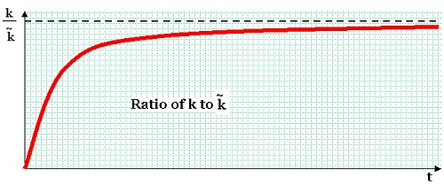
The "knife-edge", thus, means that the steady-state growth path is unstable: the only stable growth path, the "knife-edge", is where the real growth rate is equal to s/v permanently. Any slight shock that will lead real growth to deviate from this path ensures that we will not gravitate back towards that path but will rather move further away from it.

That is an unacceptable knife-edge condition, since it describes conditions that are unrealistic. But there is another case of a knife-edge equilibrium that is wide-spread and accepted in the world of economic theory: the Ramsey-Cass-Koopmans Model:


Click for larger image
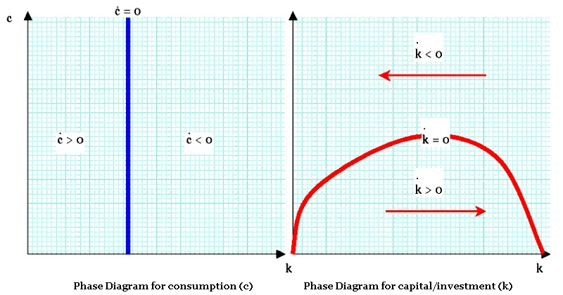
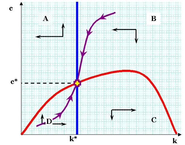
In the diagram above, k refers to the level of capital per worker in the economy, and c refers to the rate of consumption (per worker). The red curve shows all the combinations of k and c that ensure a steady rate of consumption, while the vertical blue line indicates a fixed value of k*; levels of consumption that do not sustain this pool of [depreciating] capital will lead to a steady drift of k to the left, i.e., to ever-lower levels of k. If savings is too high—and consumption too low—then k will accumulate faster.

Consider the red line a bit. If k is at or about zero, then c must be very close to zero because output (y) will be infinitesimal. If k is about midway between 0 and k*, then c must be extremely small—not merely because total output will be small, but also because c/y must be small enough for k to grow faster than the population growth rate and the rate of capital depreciation. But as we reach k*, we can loosen the belt and live a little, because the rate of capital accumulation (∆k/k) only needs to match the rate of capital depreciation and population growth in order to stay the same. If k is, say, midway between k* and the far right of the graph, then capital depreciation becomes enormous, and the rate of capital replacement becomes prohibitive. Yes, k is growing but depreciation will grow even faster than y, and the rate of consumption that is consistent with steady-state growth begins to shrink. Logically, y also declines, since investment opportunities have shrunk as well. Eventually, there is some point where k is so huge that depreciation is equal to GDP.

Now look at the purple line with the arrows. Mathematically, that's the path of stable approach to the desiderata of stable consumption and stable capital stocks. At (c*, k*), capital is replaced at a rate identical to population growth plus depreciation, and y is sufficiently high that this can be done while maintaining a steady rate of consumption. And if one is on the purple line, but not at (c*, k*), then one automatically proceeds to that point. If one off the purple path, the immediate short-term effect is one moves away towards oblivion. However, there's a difference here. The chart is not fate, but a map of derivatives; it's known as a phase diagram. According to the RCK model, people are assumed to be optimizing. In other words, if you wandered off the purple path, you would immediately notice something was wrong because the slope looked really ugly, and you'd wander back. The assumption that humans are maximizing under constraints is built into the model.

(NOTE: I am not endorsing the RCK model, which is designed as an explanatory instrument anyway; I'm merely explaining the distinction between it and other forms of knife-edge equilibrium.)

The Rational Expectations Hypothesis (REH)

The Rational Expectations Hypothesis (REH) emerged in the early 1960's as a set of theories about the financial markets. At that time, the prevailing economic theory was Keynesianism, which had evolved massively since 1936 without much supervision from its namesake. The crucial departure of Keynesianism can be summarized as "imperfect markets," which meant,

• prices may "never" adjust to reflect the intersection of supply & demand;
• money is not neutral (i.e., disinflation or deflation has a serious impact on economic conditions; the available money supply, accompanied by a distinct market for cash balances, has an impact on real output);
• factor markets, such as for labor, land, and capital, may sometimes not clear;
• state intervention may sometimes cause more good than harm.

The last proposition is a bit difficult for some people to understand. Keynes had sought to establish a macroeconomic role for the state precisely so it could avoid a microeconomic (i.e., socialistic) one, and he attempted to establish clear, immutable boundaries for the state under conditions of economic emergency.

In the period 1946-1980, economists influenced by Keynes' system (and more decisively, by his apostles) devised a framework of economic research and policy methods that bypassed any assumption of an equilibrium. There was understood to exist a microeconomic realm, which included transactions among many buyers and sellers—and which was subject to familiar Neoclassical laws of economics—and there was the macroeconomic realm of inflation, interest rates, and factor employment, where a different set of laws applied. The chief divergence in this realm was that the market never completed its process of adjustment; it could easily stop "adjusting" to full-employment equilibrium without ever getting close.

The key objection to this was always in the financial markets, i.e., the markets for bonds, commercial paper, foreign exchange, or money equivalents. Specifically, Keynesianism models developed for government agencies tended to rely on assumptions of how the money markets would respond to government actions. Everyone reading this is no doubt accustomed to news reports of the Fed changing interest rates; but it's long been noted that the Fed has limited effect in that regard. Basically, if the administration is running a "structural deficit" and the national debt is expected to remain on a permanent upward trajectory, then a reduction in the federal funds rate (the shortest-term and lowest interest rate of all) will very likely lead to an increase in longer-term rates. This was interpreted as evidence that investors make purposeful, and therefore, rational, decisions.

From there, the REH evolved to encompass a greater scope of economic behavior. After all, money markets merely respond to professionally anticipated demand for money or credit. The real sector of the economy, the part that actually does stuff, also makes plans based on inflationary expectations. At this point, the departure from pre-1979 macroeconomics becomes a little more vivid. Whereas, Keynesian economics uses simple charts to map the entire economy (IS-LM; AS-AD), REH models abandoned such visually appealing charts. Instead of graphs linking liquidity preference to interest rates and real output (the LM curve), post-Keynesian analysis relies on modeling the utility-maximizing behavior of a representative individual through time, given certain limiting assumptions: savings occurs at the expense of consumption; labor occurs at the expense of leisure; taxation influences economic activity, and most importantly, strategies to save and work are guided by expectations of the future.

The behavior of an agent in response to economic conditions is represented as a mathematical equation, nearly always the Ramsey-Cass-Koopmans Model. The RCK model is pretty flexible, and any student can edit its objective or constraint functions to reflect new hypotheses. The purpose of doing so is to create a precise map of what happens when something happens to the prevailing conditions: a change in interest rates, a scheme of fiscal stimulus (deficit spending), or central bank interventions. The RCK model is the backbone of dynamic general equilibrium (DGE) schools of economic thought, which incorporate varying degrees of REH.

However, it is not correct to claim that all this was alien to Keynesian economics. The RCK model clearly evolved in the employ of David Cass (1965) and Tjalling Koopmans (1965), both of whom were addressing questions of long-term economic growth. Neither were concerned with fiscal or monetary policy; however, it is true that by assuming economic growth was, in effect, a function of capital accumulation, both were certainly reverting to a world in which aggregate demand was not an issue. Keynes himself devoted a chapter of the General Theory to the role of expectation in business cycles. But he did not consider expectations to be so sensitive as to respond reliably to plausible state policies, and so his exposition deals exclusively with the role of the business cycle. Not surprisingly, whereas REH tended to think expectations were something business planners used to combat the state (the "policy ineffectiveness propositions"), Keynes saw expectations as undermining the neoclassical assumptions of a self-correcting economy. Hence, Keynes' use of [adaptive] expectations tended to support the idea of fiscal and monetary policy, in contrast to the REH's school's position that [rational] expectations make both pointless.

Because REH assumptions could be adjusted within the DGE schema, economists have been free to tweak them to fit the available data. However, there have been grave shortcomings in the REH results. First, the REH predictions are especially resistant to falsification. The problem is that the algorithm for selecting coefficients on any RCK equation are determined from the historical data one is trying to fit. In my opinion, this is mere data mining. It's an adaptation of the statistical procedure called regression analysis, except that the procedure is also supposed to identify "technology shocks," or disruptive events that cause spikes in the steady growth of the economy.

Let's consider these technology shocks: a contentious matter in the early days of REH, skeptics asked for examples of them. REH proponents appealed to the principle of positive economics, arguing that the point was that their model explained what actually occurred, so technology shocks were merely stylized facts. But surely there would have been a body of literature on these all-important nodes in history, particularly as REH models tended toward a standard set of assumptions. Since no such equilibrium has occurred, each version of REH produces a different set of technology shocks. One could reasonably have expected the luminaries of the field to furnish a list of the greatest shocks, and some discussion of how they affected existing technology. Instead, the official story remains the same: it's a stylized fact, don't look at it.

Stylized facts are an understandable shorthand, but when they are constantly edited so the theory fits the observations, they don't converge to a stable version of reality. Instead, they lurch about every time the data set is increased, as with the passage of time. For this reason, I would have to say that I don't expect REH to perform better in a Bretton Woods-style crisis than Keynesianism did.

---

Structural Deficit: given a fixed tax code, fixed entitlement policies, and a roughly stable rate of direct government purchases of goods & services (G), a recession will cause tax revenues to fall and government expenditures to rise. This creates a deficit (or reduces the surplus, if there was one). Conversely, if the economy is in recovery, tax revenues rise and expenditures fall, causing the budget deficit to shrink or even move to a surplus.

An incoming administration has no control over the business cycle, and has little (if any) control over the duration of its tenure. Rhetoric aside, changes to the tax code or favorable trade agreements have effects over only long periods of time. So an administration that comes to office at the beginning of a recession may defend its deficit spending by pointing out that the state is structurally in balance; i.e., the inevitable recovery will bring with it a return to fiscal balance. The point is not trivial; if the deficit is structural, then money markets will have to assume that the state's growing debts will lead both to a higher demand for credit, and higher tax rates further off in the future.

Those interested in the so-called "Ricardian Equivalence Hypothesis" of Robert Barro, please note that one study of the historical evidence established a split between the structural and non-structural elements of deficits: non-structural deficits don't stimulate increased saving.

Stylized facts: a presentation of an empirical finding, usually in statistical format. An example is the result of a regression analysis, which might correlate many variables with GDP growth. One of the variables could be a dummy variable for "Protestant majority," which might have a positive coefficient; the stylized fact here is, "there's some favorable impact on economic growth from having a Protestant majority." But it's not a universally valid generalization; it depends on what explanatory variables one used, and what the data set was. Unless the data set is relevant to the conclusions one hopes to draw, it's not useful information.

When a regression analysis is done well, it will produce a set of stylized facts that, while individually inconsequential, can be used as a group to produce valid inferences. One of the arguments used by REH theorists is that, sure, their assumptions may be individually absurd, but as a rich system of equations, they are powerful analytical tools that produce useful results. Hence, a point-by-point rebuttal of REH assumptions is an exercise in futility.

---

ADDITIONAL SOURCES & READING:

• Fabià Gumbau‐Brisa, "Heterogeneous Beliefs and Inflation Dynamics: A General Equilibrium Approach" (PDF), Federal Reserve Bank of Boston (Apr 2006)
• Sergio Rebelo, "Real Business Cycle Models: Past, Present, and Future" (PDF), Working paper, Northwestern University (2005)
• Marvin Goodfriend, "The Monetary Policy Debate Since October 1979" (PDF),
  Federal Reserve Bank of St. Louis Review, (2005)
• Marco Del Negro & Frank Schorfheide, "Priors from General Equilibrium Models for VARs" (PDF), Federal Reserve Bank of Atlanta (July 2003)
• Thomas J. Sargent, "Rational Expectations," Library of Economics & Liberty (date unknown)
• V.V. Chari, "Time Consistency and Optimal Policy Design" (PDF) Federal Reserve Bank of Minneapolis Review (1988)
• Thomas J. Sargent, "Rational Expectations and the Reconstruction of Macroeconomics," Federal Reserve Bank of Minneapolis Review (1980)

BOOKS: Roger Guesnerie, Assessing Rational Expectations, MIT Press (2001); Stephen M. Sheffrin, Rational Expectations, 2nd Edition, Cambridge (1996); Preston Miller (editor), The Rational Expectations Revolution, MIT Press (1996);

Dynamic General Equilibrium

The dynamic general equilibrium (DGE) model of economic behavior is the one that has prevailed in public policy analysis for about 30 years now. In its early form, it tended to use, and was known as, the "rational expectations hypothesis" (REH) ; and a money-neutral version of the business cycle, or "real business cycle" (RBC) theory. In the years since, there has been a shift of emphasis away from REH and RBC, towards the design of the model itself (DGE). Hence, DGE methodology can specifically exclude some of the early assumptions, and incorporate their converse.

When students are introduced to the concept of equilibrium, what they are are shown is the intersecting schedules of supply and demand. A leftward shift in the supply curve—perhaps due to the depletion of a particular input—causes the price to rise and the quantity demanded to decrease. A rightward shift in the demand curve—perhaps due to a change in fashion—also causes prices to increase, but also causes the quantity demanded to increase too.


This is known as a partial equilibrium, since only a part of the determinants of the equilibrium are being looked at. In fact, professors are obligated to remind students that these conditions hold, "all other things being equal." If the supply curve moves to the right, we don't consider a sudden decrease in income, or a sudden shift rightward in the supply curves of other commodities.

Initially, the concept of general equilibrium appears to have been developed by Leon Walras (1870), and subsequently refined by Gustav Cassel (1918). Walras' original version did not fare well, but in the 1950's was revived by Kenneth Arrow and Gerard Debreu, and since then general equilibrium has evolved to become the essential governing idea of economic research.

In general equilibrium, all of the determinants of economic equilibrium are considered at once. This can be gone though a system of linear equations. The equations incorporate the utility functions of representative consumers, prior endowments of capital and labor, production functions (i.e., equations that provide the maximum output of commodities for an economy, given available labor and capital; see Egwald), and so on. The object is to create a mathematical representation of how an economy works.

Why?
Part of the reason is to examine the more complicated results of external change. For example, in intermediate microeconomics, students are typically introduced to indifference curves and budget lines. This allows students to analyze the difference between the income effect and the substitution effect (both of which involve changes in demand caused by changes in price). But the curves in the textbooks are usually drawn arbitrarily, to make a particular point; Marshallian general equilibrium theory tended to resist integrating all of the elements of Neoclassical (Marginalist) theory into a formal, mathematical model.

Colander: Why did Marshall focus his analysis on partial equilibrium and not formally develop his conception of general equilibrium? [...] I think it is correct that he felt incapable of specifying a meaningful formal general equilibrium system, [...] because he demanded intuitive correspondence between math and his understanding of the economy. [...]

Marshall's recognition of the analytic intractability of the general equilibrium problem, given the math available to him, and his desire for concreteness in his economics, led him to shy away from abstract specifications of general equilibrium.

However, the work of Arrow and Debreu was to effectively synthesize the views of Marshall with Walras' (inter alia) notions of general equilibrium. In other words, Marshall's partial, "cross sections" of economic relations (like the indifference curve) are expanded into the additional dimensions required to allow for a formal, unique equilibrium for any given vector of determinant variables—capital and labor endowments, consumer preferences, technology (production functions) and so on.

A word on simplification: in order to represent something as complex as an entire economy with a series of linear equations, economists typically rely on a principle known as positive economics. Positive economics, in its most reduced form, merely asks that economic analysis be judged on the basis of its accuracy of predictions, rather than normative (value) judgments. An interesting corollary to this is that we are advised to consider an economic theory on the basis of its predictive performance, rather than the realism of its assumptions[*]. Hence, we might assume that the US economy consists of 300 million identical actors, rather than people varying widely in income, ability, or preferences. We might ignore the role of monopolies, or involuntary unemployment, or ignorance about the relevant policy preferences of monetary authorities, and that's all right, if the result provides a reasonably accurate or useful prediction of the future.

Variations on a Theme
As mentioned above, DGE theory initially incorporated mathematical equations that "assumed" no liquidity constraints, rational expectations hypothesis (REH), and real business cycles (RBC). Initially, REH was considered to be identical to DGE, which is why you find all of the DGE ideas expressed in The Rational Expectations Revolution (cited below); Preston Miller's book wasn't entitled The Dynamic General Equilibrium Revolution, although six years later it might well have been: since 2001, usage of the term has sharply diminished.

Moreover, there are different systems of equations that may be used. The most common are those of the Ramsey-Cass-Koopmans model: the closed economy consists of a household with an exogenous labor supply over time. One good is produced in each period using inputs of labor and capital, and output in each period can be either consumed or invested. There is perfect competition in all markets and no taxes. Individuals are assumed to have an infinite horizon, and expectations by private agents are forward-looking and rational. Hence, all agents have perfect foresight because there is no uncertainty. These assumptions imply that the allocation of resources by a central planner who maximizes the utility of the representative agent is identical to the allocation of resources in an undistorted decentralized economy.

The dynamic component comes from the use of mathematical models to simulate the behavior of such an economy over time (an innovation of Edward C. Prescott's "Time to Build" paper, cited below). In such a model, the economy has predictable responses to various kinds of external shocks ("technology shocks"), each of which corroborate the others.

DGE models that incorporate assumptions of perfect market conditions and optimal agent responses tend to rely entirely on random ("stochastic") shocks to explain everything that actually happens. Some researchers, such as Edward C. Prescott, have sought to create simulations of an economy that replicate the behavior of the actual economy.

---

ADDITIONAL SOURCES & READING: CEPA New School of Economics, "The Neo-Walrasian General Equilibrium System"; David Colander, "Marshallian general equilibrium analysis (PDF)," Eastern Economic Review (1995);

Red typeface indicates available through JSTOR

• Sergio Rebelo, "Real Business Cycle Models: Past, Present, and Future" (PDF), Working Paper, Northwestern University (2005)
  
• Marvin Goodfriend, "The Monetary Policy Debate Since October 1979" (PDF),
  Federal Reserve Bank of St. Louis Review, (2005)
• Sergey Paltsev, "Moving from Static to Dynamic General Equilibrium Economic Models (Notes for a beginner in MPSGE)" (PDF) Joint Program on the Science and Policy of Global Change, MIT (June 2004)
  
• Jesus Fernandez-Villaverde & Juan Francisco Rubio-Ramírez, "Some Results on the Solution of the Neoclassical Growth Model" (PDF), Federal Reserve Bank of Atlanta (Dec 2003)
• Marco Del Negro & Frank Schorfheide, "Priors from General Equilibrium Models for VARs" (PDF), Federal Reserve Bank of Atlanta (July 2003)
• Morten I. Lau, Andreas Pahlke & Thomas F. Rutherford, "Modeling Economic Adjustment: A Primer in Dynamic General Equilibrium Analysis," University of Copenhagen, University of Stuttgart, University of Colorado@Boulder (1997)
  
• Federal Reserve Quarterly (Fall-1986)
  • Rodolfo E. Manuelli, "A guide to the Prescott-Summers Debate" (PDF)
  • Edward Prescott, "Theory Ahead of Business Cycle Measurement" (PDF)
  • Lawrence H. Summers, "Some Skeptical Observations"
  • Edward C. Prescott, "Response to a Skeptic" (PDF)
• Finn E. Kydland & Edward C. Prescott, "Time to Build and Aggregate Fluctuations," Econometrica (1982).
• Robert Lucas, "An Equilibrium Model of the Business Cycle," Journal of Political Economy—University of Chicago (1975)

BOOKS: David C. Colander, Post Walrasian Macroeconomics: Beyond the Dynamic Stochastic General Equilibrium Model, Cambridge University Press (2006); Stephen M. Sheffrin, Rational Expectations, 2nd Edition, Cambridge (1996); Preston Miller (editor), The Rational Expectations Revolution, MIT Press (1996);

The Dynamics of Industrial Choice (3)

(Part 1 and 2)

In Part 2 we had a brush with the basic classical economic growth model. The model in question has come in for a significant amount of criticism, not least because it assumes constant full employment (in the sense that unemployment is ALWAYS a choice people make), no significant effect of monopolies, and unlimited ability to defer consumption.

An issue I have with the model is that, ironically, it suppresses the truth it reveals. Technology it treats as absolutely nothing more than the disaggregated residual of economic growth, after subtracting capital and labor growth. The model mentions firms, but they have no objective function to maximize; they aren't constrained by prior technology; they aren't tied to formats. They simply provide a ratio between inputs and output; but both are homogeneous. In plain English, they assume the economy behaves like a gas, not something lumpy. Usually, when you use a mathematical model, it's simplified because there are obvious limits to the complexity of the math one may do. The model may describe optimal conditions for event x, for proving x is impossible even under the most favorable of conditions. Conversely, one might prove the inevitability of x by demonstrating that, even under the most restrictive of conditions (so restrictive they're practically impossible), x will still happen anyway. A third purpose is to show hypothetical conditions under which x could conceivably happen, even though the frequency of those conditions is subject to further inquiry. The RCK model does none of these things.

However, the RCK model can be modified to depict different things entirely. It is not very good at modeling the aggregate economy.* It is somewhat better as a conceptual tool in explaining the forces acting on actors like firms (not households). Households are too varied in character; they are too numerous; and their dynamics of maximization are incompatible with the assumptions of the RCK model. Firms can be grouped into plausible categories based on stranded costs and capital structure; in contrast, households may or may not be constrained by subsistence constraints, multiple members, perverse incentives, and unknown optimization strategies. On the other hand, firms have clear optimization goals.

Additionally, the optimality analysis for which Frank Ramsey had originally suggested his model, is a more reasonable application of the RCK model anyway. In this case, the object is to evaluate the optimality of decisions, not to make predictions or deductions of the "actually existing" economy. Such optimality information about households is, to reiterate, useless; about firms, it can be used to evaluate policy of firm administration. Corporations, with legal powers of limited liability and access to "capital markets," are, in some senses, surrogates of the state. Banks, for example, are a category of firm who are empowered to create money. Their governance is therefore a valid target of this sort of analysis.

A second modification I would recommend pertains to the objective functions that our economic agents seek to maximize. In the original RCK, if the economic actor is off the sadddle point, then it will increase savings to precisely that level required for path-convergence. Yet the functions of capital accumulation out of personal accumulation are pushing in the opposite direction; the situation can be likened to a pedestrian running frantically up a down escalator. That the escalator always points in the direction away from the equilibrium growth position, is an awkward but inevitable fact of the household savings-consumption equation; the optimization function requires that the household will [on average] react by running up the escalator faster than the escalator is moving. From experience, we know this is not true for firms, whose existence takes a clear trajectory from expansion to stagnation to financial collapse.

Corporations manufacturing a particular item are motivated to maximize earnings out of revenues. But rather than following a steady-state optimization function, they have a trajectory, or path through time. Rather than assuming the corporate management optimizes its capital structure and technology choices for a steady state growth, which is unrealistic, we would instead plot the firm as responding to conditions at any moment based on its optimization function, the capital structure, and stranded costs. Firms achieve optimization by selecting between quality and quantity (i.e., between improving processes and enlarging scale). Improved processes result in at least two positive feedbacks: higher revenues (which may persist, longer than the costs of transition to the improved process did) AND lower stranded costs (since the process is revived repeatedly, so stranded costs are reduced in the process design).

I would expect a mathematical exposition of this would reveal that, where market share is basically fixed, quality and low stranded costs would become the preferred choice; and capital structure would tend towards debt, rather than equity.
___________________________________________________
SOURCES & ADDITIONAL READING: Douglas J. Puffert, "Path Dependence, Network Form, and Technological Change" (PDF); Kenneth J. Arrow, "Path Dependence & Competitive Equilibrium" (PDF); David F. Weiman, "Building ‘Universal Service’ in the Early Bell System: The Reciprocal Development of Regional Urban Systems and Long Distance Telephone Networks" (PDF).
___________________________________________________
* That the RCK model does not describe observed reality is demonstrated by empirical comparisons of predictions of inflation, interest rates, prices of specific commodities, and so forth. A survey of the historical evidence is found in Steven M. Sheffrin's Rational Expectations. Moreover, the RCK model predicts fairly rapid rates of convergence for economies with disparate levels of productivity—provided trade barriers are low. Convergence of productivity and capital stocks among the economies of the world have not remotely matched expectations. No one has ever tweaked the RCK parameters or equations to provide reasonably accurate predictions of fluctuations of savings or capital (this has been acknowledged by the PDF files explaining the RCK model, linked in part 2.) The same is true for David Romer's Advanced Macroeconomics. Hence, the RCK does not make reasonably accurate predictions about the performance of different economies in the world.

The Dynamics of Industrial Choice (2)

(Part 1)

Industries make decisions about the implementation of technologies according to expected returns of that implementation: that's the standard position of orthodox economic theory. The reality is more complex, but it's interesting to see how even the very simple, reductionist mathematical models used to simulate the behavior of a simple economy lead to complex systems.

Since the basic rules of economic explanation are relatively simple, efforts have been made many times to reduce these to mathematical formulas that can describe the workings of a system. One idea has been to use these to re-create the laws of motion that prevail in an economy, so that the rules can be refined based on their predictive powers. The best-known attempt to do this has been the Ramsey-Cass-Koopmans Model, which simplifies the job by treating the economy as if it consisted of a single, average household.

The RAMSEY-CASS-KOOPMANS MODEL
Attributes of the household are inherent in the economic system. Households have endowments of labor (l) and capital (k). Labor is paid at wage w and capital commands an interest rate r. Hence, the income (y) of the household will be

y = wl + rk. However, while the endowment k accrues interest without labor, it also depreciates at rate δ; presumably r < δ, or else there would be little point in holding k. Likewise, L is accumulated from y - c; in the RCK model, all income that is not immediately consumed is saved, and therefore invested in the form of more k.

In economics, K always represents the total stock of capital; k (small) represents the supply available to our sample household at any moment in time. The symbol ρ stands for the discounting of future consumption; economists assume that consumers value future consumption less than present consumption.¹ Stocks of capital depreciate at a rate of δ, so they must be replaced at a rate of δk. There must also be a rate of return on capital, which is r; it's common to assume that r = ρ + δ, since (by definition) if r < ρ + δ, people would be irrationally postponing consumption, and if r < ρ + δ, people are irrationally improvident. Each household is intuitively driven to maximize the equation below.
This is not as far fetched as it might seem. That's because the "average" path taken by millions of households groping towards an optimal allocation may well fit this description. Groping comes in the form of endless brushes with frustration and lost opportunities. Errors or eccentric decisions made by this or that individual may be expected to average out over very large numbers and over great lengths of time.

The household stock of capital increases at rate , which will be
= (r – δ)k + wl - c
There is a consumption function U(C) is assumed to take the form below:

This is the function for constant relative risk aversion (CRRA); it is also known as the continuous intertemporal elasticity of substitution (CIES) function. Since we do not impose a time horizon, there's a risk of what is called a "corner solution," which is where the maximum point of a function lies at one limit or the other of its domain. The danger here is that the solution would be "c = 0" for all t < ∞, since ∞ is the biggest number we have. At the end of time, k_∞ would be extremely large, but the who affair would be utterly pointless since our whole effort to simulate the economy with an average household would lead to that household acting in accordance with totally arbitrary equations. Such a scenario is unreasonable; people have to consume something even when their incomes are so low they can save scarcely anything, so we have limits to the value of infinitely postponed consumption.

The economy also incorporates an average firm, which transforms l and k into y. Beyond this, however, the firm does not appear; it does not have an objective function to maximize, for instance; it is not in conflict with other firms or the representative household. The RCK is an extremely adaptive model, however, and a very large number of variations on it exist. Here, we'll be sticking to the plain vanilla version.



Click for larger image

This chart shows the two phase diagrams in the RCK model. On the left, the blue line represents constant, stable rates of consumption; c-dot represents the 1st derivative of c(t) with respect to time. Let's say that k* represents the point on the horizontal axis where c-dot = 0 (where the blue line touches the bottom edge). Then levels of capital endowment k* leads to a decrease in consumption.

(Please note that c-dot is instantaneous. I point this out because, if one occupies a position {k0, c0} , then one will presently move to another point on the phase diagram.)

On the right, the red curve indicates all the positions where k-dot is 0; if one occupies positions along that line, one's net growth in capital endowments is zero. For values of c above the red line, one's rate of capital accumulation is negative (one is spending out of one's substance!). For levels of c below the red line, one's rate of capital accumulation is positive, because one is consuming so little.



Click for larger image
Here, the two maximization functions are combined. Where the red and blue lines intersect, there is steady state consumption and capital endowment. At points along the violet line passing through the intersection, points are not in equilibrium, but are "gravitating" towards it.

The economy (in the avatar of its representative households) is has a peculiar version of the knife-edged equilibrium. The saddle equilibrium might appear to suggest that the economy, if perturbed from perfect order, would plunge into wreckage, like a locomotive on a tightrope. Over the short-run, as during recessions, this would appear to be the case; and over very long periods of history, flourishing economies do eventually enter periods of decline. However, the RCK model pertains to medium-run trends; the model is not, nor ever could be, rich enough to capture the multifarious forces of the short-run, and over the long-run things such as civil wars, obsolete institutions, demographic changes, and so forth are simply out of the model.

The other important distinction is that when an economy is not on the violet line in the graph above, the optimization preferences of its population will tend to push it toward convergence with the steady-state, balanced growth economy. In fact, the model incorporates projections of how this occurs.


In the graph above, the economy responds with a reduction in consumption, and concomitant increase in saving. Richer models incorporate a "floor" of consumption that causes it to start low, and rise to overshoot the higher balanced growth path (BGP) savings rate.


Here, the economy's stock of capital is converging. Notice that the high saving rate is accompanied by a steep slope for k; high values of s amount to exactly the same thing as high values of . Likewise, in our simplified model, the efforts of households to maximize consumption over infinite time horizons leads to rapid accumulation.


This is the big picture: the balanced growth curve, in which the endogenous factors are growing at a constant pace (dotted line) while the equilibrium growth path gradually catches up.

(Part 3)
____________________________________________
Notes

1 Time discounting: it is usually assumed that humans generally prefer consumption in the present to consumption in the future. As a result, we assume humans have to pay more to consume now than they do if they wait.  Discounting is a way of expressing this preference in the form of a low price for future consumption.

As always, special exceptions may apply but remember, economists tend to be interested in average or median behavior. Even if exceptions are very common, therefore, people with unusual time-of-consumption preferences can demand the same discount as everyone else.

Typically, for purposes of government accounting the Office of Management and Budget (OMB) uses a rate of 7%, and tests for rates of 5%-9%.
____________________________________________
Resources and Additional Reading:

The Ramsey-Cass-Koopmans model is explained formally here (and here), for those of you interested in a backup source. The first link is to the site of Prof. Thomas M. Steger in Zurich; in my opinion, his explanation is not only the best I've seen online (and the most reliable), it's also better than the one in David Romer's textbook Advanced Macroeconomics (1st edition), which is the one I was initially using. Juan Ruiz, a Spanish economist, posted lecture notes on the RCK model that are also very easy to follow.

For a detailed introduction to production functions, see Egwald Economics;