Constant Relative Risk Aversion

There is a game of chance called "St Petersburg," which is the simplest thing possible. Take a fair coin and flip it. You have bet 2 rubles on the outcome. If the coin comes up heads then you win 2 rubles, but if it comes up tails you play again, this time for 4 rubles. Each time, the stake is doubled, so n plays yields a prize of 2ⁿ rubles. Each flip of the coin is called a "trial" and the string of trials with their outcomes that concludes the game, is called a "consequence."

The probability of a consequence of n flips ('P(n)') is 1 divided by 2n, and the "expected payoff" of each consequence is the prize times its probability. The ‘expected value’ of the game is the sum of the expected payoffs of all the consequences. Since the expected payoff of each possible consequence is 1 ruble, and there are an infinite number of them, this sum is an infinite number of rubles. This became known as the St. Petersburg Paradox.

Bernoulli, the Swiss philosopher and mathematician, suggested the problem lay in rewarding people with money rather than utility. At the back of the paradox is the assumption that (2ⁿ)(2^-n) = 1 for all values of n; as n becomes (or could become) infinitely large, the sum of probable outcomes reaches ∞. In fact, that's not true for utility, and Bernoulli proposed that the expected utility--as opposed to expected payout in rubles--was necessarily finite.¹

Economists were increasingly interested in risk² because it applies to virtually all decisions, particularly those related to savings. Suppose you have a temporary employee working at a longterm assignment. The temp could be dismissed at any second; temps are almost never given any notice, and an abrupt dismissal typically causes the temp a lot of hardship. Because of this, the temp faces a risk if she accrues any debt; savings are vital to surviving periods between assignments. Yet there is also potential benefit in taking night school courses--say, in accounting. She must therefore weigh the risk (weighted for consequences) of dismissal, against the probability of getting a permanent job with benefits (weighted for the benefits of doing so).

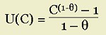
Putting this another way, let U be the utility experienced by the temp. U is a function of consumption C, which of course varies over time; U = U(C(t)). The temp may prefer to take risks in order to enhance her estimated future consumption: an increase in income caused by risky investment of scarce money in tuition. For small values of θ, marginal utility diminishes more slowly--i.e., U˝(C) is smaller--than for larger values. That's the crucial significance of θ.

In the equation above, a high value of θ signifies that the consumer is quickly sated by increasing consumption. Hence, both high values of consumption all at one time, and a high payoff from a high risk bear less gratification, than would be the case if θ were low. Hence, another term for "constant relative risk aversion" is "constant intertemporal elasticity of substitution" (CIES). On average, the tendency to accept risk (in exchange for a payoff) and the tendency to accept a major belt-tightening (in exchange for a future payout) are comparable.

In the graph below, the horizontal axis C(z) refers to a random outcome; the probability that z₁ happens is p, and the probability that z₂ happens is (1-p). In other words, either z₁ or z₂ can happen. So the expected outcome E(z) is pz₁ + (1-p)z₂. Now, please notice someone has drawn a chord between points A and B. Notice that the expected utility E(U) is substantially lower than the utility of the expected outcome u[E(z)]; or just notice D and E. The position of E on the chord is dependent on the ratio of p:(p-1).

The behavioral inference drawn from this chart is that the utility of expected income U[E(z)] is greater than the expected utiliy E(U), i.e.,

U[pz₁ + (1-p)z₂] > Upz₁ + U(1-p)z₂
This is just a complicated way of saying that risk aversion inflicts a severe hit on the utility of bundle of benefits.

The function above was developed by Milton Friedman and Leonard Savage in 1948. Friedman & Savage also speculated on other shapes of the risk-utility function, but the curve above has a certain usefulness for the economics profession. You see, if a person has a curve very much unlike the one shown above, then one can be presented with a series of risks, each of which one finds acceptable, that lead one into any position; the other party--say, the casino management--can always make a profit, and essentially "pump" money out of players. While some people undoubtedly are like that, the population in the aggregate cannot be, or the economy would grind to a halt forever.

If we are looking at the function as a CIES graph, then the horizontal access merely represents increasing values of consumption. If, however, we are looking at the function as a CRRA graph, then it makes sense to regard the horizontal axis as a series of equally likely payouts. A segment between z_i and z_j with a length of 1% of the entire horizontal axis, would have a 1% possibility of happening.
__________________________________________________
NOTES

1 For those of you unfamiliar with calculus: some algebraic functions, like f(x) = x^-2 can be graphed from 0 to infinity, and the total area under their curve is finite. This seems impossible, but it's true.

2 Risk and uncertainty are (usually) regarded as distinct topics in economics. Risk is quantifiable; uncertainty is not. Or, in the words of Frank L. Knight,

The essential fact is that "risk" means in some cases a quantity susceptible of measurement, while at other times it is something distinctly not of this character; and there are far-reaching and crucial differences in the bearings of the phenomenon depending on which of the two is really present and operating. There are other ambiguities in the term "risk" as well, which will be pointed out; but this is the most important. It will appear that a measurable uncertainty, or "risk" proper, as we shall use the term, is so far different from an unmeasurable one that it is not in effect an uncertainty at all. We shall accordingly restrict the term "uncertainty" to cases of the non-quantitative type. It is this "true" uncertainty, and not risk, as has been argued, which forms the basis of a valid theory of profit and accounts for the divergence between actual and theoretical competition.
[Risk, Uncertainty, and Profit, 1921]

The Dynamics of Industrial Choice (2)

(Part 1)

Industries make decisions about the implementation of technologies according to expected returns of that implementation: that's the standard position of orthodox economic theory. The reality is more complex, but it's interesting to see how even the very simple, reductionist mathematical models used to simulate the behavior of a simple economy lead to complex systems.

Since the basic rules of economic explanation are relatively simple, efforts have been made many times to reduce these to mathematical formulas that can describe the workings of a system. One idea has been to use these to re-create the laws of motion that prevail in an economy, so that the rules can be refined based on their predictive powers. The best-known attempt to do this has been the Ramsey-Cass-Koopmans Model, which simplifies the job by treating the economy as if it consisted of a single, average household.

The RAMSEY-CASS-KOOPMANS MODEL
Attributes of the household are inherent in the economic system. Households have endowments of labor (l) and capital (k). Labor is paid at wage w and capital commands an interest rate r. Hence, the income (y) of the household will be

y = wl + rk. However, while the endowment k accrues interest without labor, it also depreciates at rate δ; presumably r < δ, or else there would be little point in holding k. Likewise, L is accumulated from y - c; in the RCK model, all income that is not immediately consumed is saved, and therefore invested in the form of more k.

In economics, K always represents the total stock of capital; k (small) represents the supply available to our sample household at any moment in time. The symbol ρ stands for the discounting of future consumption; economists assume that consumers value future consumption less than present consumption.¹ Stocks of capital depreciate at a rate of δ, so they must be replaced at a rate of δk. There must also be a rate of return on capital, which is r; it's common to assume that r = ρ + δ, since (by definition) if r < ρ + δ, people would be irrationally postponing consumption, and if r < ρ + δ, people are irrationally improvident. Each household is intuitively driven to maximize the equation below.
This is not as far fetched as it might seem. That's because the "average" path taken by millions of households groping towards an optimal allocation may well fit this description. Groping comes in the form of endless brushes with frustration and lost opportunities. Errors or eccentric decisions made by this or that individual may be expected to average out over very large numbers and over great lengths of time.

The household stock of capital increases at rate , which will be
= (r – δ)k + wl - c
There is a consumption function U(C) is assumed to take the form below:

This is the function for constant relative risk aversion (CRRA); it is also known as the continuous intertemporal elasticity of substitution (CIES) function. Since we do not impose a time horizon, there's a risk of what is called a "corner solution," which is where the maximum point of a function lies at one limit or the other of its domain. The danger here is that the solution would be "c = 0" for all t < ∞, since ∞ is the biggest number we have. At the end of time, k_∞ would be extremely large, but the who affair would be utterly pointless since our whole effort to simulate the economy with an average household would lead to that household acting in accordance with totally arbitrary equations. Such a scenario is unreasonable; people have to consume something even when their incomes are so low they can save scarcely anything, so we have limits to the value of infinitely postponed consumption.

The economy also incorporates an average firm, which transforms l and k into y. Beyond this, however, the firm does not appear; it does not have an objective function to maximize, for instance; it is not in conflict with other firms or the representative household. The RCK is an extremely adaptive model, however, and a very large number of variations on it exist. Here, we'll be sticking to the plain vanilla version.



Click for larger image

This chart shows the two phase diagrams in the RCK model. On the left, the blue line represents constant, stable rates of consumption; c-dot represents the 1st derivative of c(t) with respect to time. Let's say that k* represents the point on the horizontal axis where c-dot = 0 (where the blue line touches the bottom edge). Then levels of capital endowment k* leads to a decrease in consumption.

(Please note that c-dot is instantaneous. I point this out because, if one occupies a position {k0, c0} , then one will presently move to another point on the phase diagram.)

On the right, the red curve indicates all the positions where k-dot is 0; if one occupies positions along that line, one's net growth in capital endowments is zero. For values of c above the red line, one's rate of capital accumulation is negative (one is spending out of one's substance!). For levels of c below the red line, one's rate of capital accumulation is positive, because one is consuming so little.



Click for larger image
Here, the two maximization functions are combined. Where the red and blue lines intersect, there is steady state consumption and capital endowment. At points along the violet line passing through the intersection, points are not in equilibrium, but are "gravitating" towards it.

The economy (in the avatar of its representative households) is has a peculiar version of the knife-edged equilibrium. The saddle equilibrium might appear to suggest that the economy, if perturbed from perfect order, would plunge into wreckage, like a locomotive on a tightrope. Over the short-run, as during recessions, this would appear to be the case; and over very long periods of history, flourishing economies do eventually enter periods of decline. However, the RCK model pertains to medium-run trends; the model is not, nor ever could be, rich enough to capture the multifarious forces of the short-run, and over the long-run things such as civil wars, obsolete institutions, demographic changes, and so forth are simply out of the model.

The other important distinction is that when an economy is not on the violet line in the graph above, the optimization preferences of its population will tend to push it toward convergence with the steady-state, balanced growth economy. In fact, the model incorporates projections of how this occurs.


In the graph above, the economy responds with a reduction in consumption, and concomitant increase in saving. Richer models incorporate a "floor" of consumption that causes it to start low, and rise to overshoot the higher balanced growth path (BGP) savings rate.


Here, the economy's stock of capital is converging. Notice that the high saving rate is accompanied by a steep slope for k; high values of s amount to exactly the same thing as high values of . Likewise, in our simplified model, the efforts of households to maximize consumption over infinite time horizons leads to rapid accumulation.


This is the big picture: the balanced growth curve, in which the endogenous factors are growing at a constant pace (dotted line) while the equilibrium growth path gradually catches up.

(Part 3)
____________________________________________
Notes

1 Time discounting: it is usually assumed that humans generally prefer consumption in the present to consumption in the future. As a result, we assume humans have to pay more to consume now than they do if they wait.  Discounting is a way of expressing this preference in the form of a low price for future consumption.

As always, special exceptions may apply but remember, economists tend to be interested in average or median behavior. Even if exceptions are very common, therefore, people with unusual time-of-consumption preferences can demand the same discount as everyone else.

Typically, for purposes of government accounting the Office of Management and Budget (OMB) uses a rate of 7%, and tests for rates of 5%-9%.
____________________________________________
Resources and Additional Reading:

The Ramsey-Cass-Koopmans model is explained formally here (and here), for those of you interested in a backup source. The first link is to the site of Prof. Thomas M. Steger in Zurich; in my opinion, his explanation is not only the best I've seen online (and the most reliable), it's also better than the one in David Romer's textbook Advanced Macroeconomics (1st edition), which is the one I was initially using. Juan Ruiz, a Spanish economist, posted lecture notes on the RCK model that are also very easy to follow.

For a detailed introduction to production functions, see Egwald Economics;