Knife-Edge Equilibrium

A condition in which something must either be at a precise equilibrium, or else tumble way into catastrophe. In some cases, such as something that really is balanced on a knife's edge, it's an accurate description. However, in models of (say) economic growth, it's a severe flaw in the model.

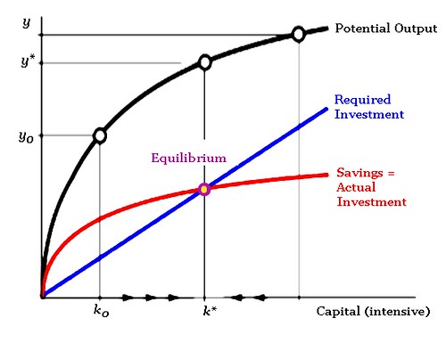
One of the most famous examples of the knife's edge equilibrium is in the Harrod-Domar Growth Model (1949), which sought to integrate some theory of economic growth with the Keynesian General Theory. Under the Harrod-Domar model, there is a precise rate of investment which is compatible with full employment.

Recall, from Keynes, that investment is one of the determinants of aggregate demand and that aggregate demand is linked to output (or aggregate supply) via the multiplier. Abstracting from all other components, we can write that, in goods market equilibrium:
Y = (1/s)I

where Y is income, I investment, s the marginal propensity to save (and thus the multiplier is 1/s). But investment, note Harrod and Domar, increases the productive capacity of an economy and that itself should change goods market equilbrium.

For "steady state" growth, in the language of Harrod-Domar, aggregate demand must grow at the same rate as the economy's output capacity grows. Now, the investment-output ratio, I/Y, can be expressed as (I/K)(K/Y). Now, I/K is the rate of capital accumulation and K/Y is the capital-output ratio (call it "v"). Thus, the rate of capital accumulation, I/K, is the rate of capacity growth (call that "g"). Thus, for steady state it must be that I/K = (dY/dt)/Y = g (i.e. the rate of capital accumulation/capacity growth, I/K, and the real rate of output growth (dY/dt)/Y, must be at the same rate, g). Thus, plugging in our terms:
I/Y = (I/K)(K/Y) = gv

But recall our goods market equilibrium term from the multiplier, i.e., Y = (1/s)I which can be rewritten I/Y = s. Thus, the condition for full employment steady-state growth is gv = s, or simply:
g = s/v
Thus, s/v is the "warranted growth rate" of output. However, Harrod and Domar originally held s and v as constants—determined by institutional structures. This gives rise to the famous Harrodian "knife-edge": if actual growth is slower than the warranted rate, then effectively we are claiming that excess capacity is being generated, i.e., the growth of an economy's productive capacity is outstripping aggregate demand growth. This excess capacity will itself induce firms to invest less—but, then, that decline in investment will itself reduce demand growth further—and thus, in the next period, even greater excess capacity is generated.

Similarly, if actual growth is faster than the warranted growth rate, then demand growth is outstripping the economy's productive capacity. Insufficient capacity implies that entrepreneurs will try to increase capacity through investment—but that that itself is a demand increase, making the shortage even more acute. With demand always one step ahead of supply, the Harrod-Domar model guarantees that unless we have demand growth and output growth at exactly the same rate, i.e., demand is growing at the warranted rate, then the economy will either grow or collapse indefinitely.

The "knife-edge", thus, means that the steady-state growth path is unstable: the only stable growth path, the "knife-edge", is where the real growth rate is equal to s/v permanently. Any slight shock that will lead real growth to deviate from this path ensures that we will not gravitate back towards that path but will rather move further away from it.

That is an unacceptable knife-edge condition, since it describes conditions that are unrealistic. But there is another case of a knife-edge equilibrium that is wide-spread and accepted in the world of economic theory: the Ramsey-Cass-Koopmans Model:


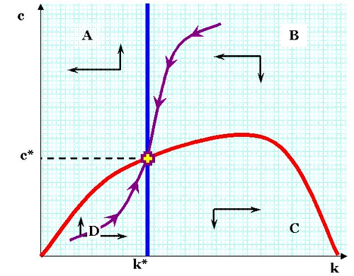
Click for larger image
In the diagram above, k refers to the level of capital per worker in the economy, and c refers to the rate of consumption (per worker). The red curve shows all the combinations of k and c that ensure a steady rate of consumption, while the vertical blue line indicates a fixed value of k*; levels of consumption that do not sustain this pool of [depreciating] capital will lead to a steady drift of k to the left, i.e., to ever-lower levels of k. If savings is too high—and consumption too low—then k will accumulate faster.

Consider the red line a bit. If k is at or about zero, then c must be very close to zero because output (y) will be infinitesimal. If k is about midway between 0 and k*, then c must be extremely small—not merely because total output will be small, but also because c/y must be small enough for k to grow faster than the population growth rate and the rate of capital depreciation. But as we reach k*, we can loosen the belt and live a little, because the rate of capital accumulation (∆k/k) only needs to match the rate of capital depreciation and population growth in order to stay the same. If k is, say, midway between k* and the far right of the graph, then capital depreciation becomes enormous, and the rate of capital replacement becomes prohibitive. Yes, k is growing but depreciation will grow even faster than y, and the rate of consumption that is consistent with steady-state growth begins to shrink. Logically, y also declines, since investment opportunities have shrunk as well. Eventually, there is some point where k is so huge that depreciation is equal to GDP.

Now look at the purple line with the arrows. Mathematically, that's the path of stable approach to the desiderata of stable consumption and stable capital stocks. At (c*, k*), capital is replaced at a rate identical to population growth plus depreciation, and y is sufficiently high that this can be done while maintaining a steady rate of consumption. And if one is on the purple line, but not at (c*, k*), then one automatically proceeds to that point. If one off the purple path, the immediate short-term effect is one moves away towards oblivion. However, there's a difference here. The chart is not fate, but a map of derivatives; it's known as a phase diagram. According to the RCK model, people are assumed to be optimizing. In other words, if you wandered off the purple path, you would immediately notice something was wrong because the slope looked really ugly, and you'd wander back. The assumption that humans are maximizing under constraints is built into the model.

(NOTE: I am not endorsing the RCK model, which is designed as an explanatory instrument anyway; I'm merely explaining the distinction between it and other forms of knife-edge equilibrium.)

Cerebus to take Chrysler off Daimler's Hands

Today, a leading story is that Cerebus Capital Management has agreed to pay $7.4 billion for the Chrysler Group. With cash infusions by DaimlerChrysler of greater than $8.1 billion (€6.0 billion), this means the future-former DaimlerChrysler is coughing up a net $700 million. In 1998, Chrysler was a robust company in its fourth year of flourishing recovery. It held 23% of the North American market for cars and trucks and was regarded as a potential white knight for tottering Korean automakers.

Instead, that year, Daimler-Benz CEO Jürgen Schrempp added the number 3 US automaker to his reliquary of overseas acquisitions. Schrempp was well-connected and famous for his iconoclastic (for Germany) practice of high-flying aggressive M&A activity. He had already bought American LaFrance (PDF) and Fokker, sunk billions of marks into the latter, and skuppered it (1996). Schrempp had led the South African division of Daimler-Benz in the early 1980's before taking over DB's airspace division, DASA, in 1989. Here, he won a reputation as the architect of DASA's transformation from a gigantic European aerospace corporation into EADS.* In 1995 he took over the parent company, Daimler-Benz; the following year, DASA gave up on Fokker.

Schrempp had promoted the M&A with Chrysler as "a merger of equals"; after telling an interviewer for the German newspaper Handelsblatt that he had always intended for Chrysler to be a division of Daimler-Benz, investor Kirk Kerkorian sued Schrempp for misleading shareholders about his intentions.** But this was the least of his worries. Nine years later, in a period of soaring share prices for the largest industrial firms, the market value of DaimlerChrysler was about the same—$44 billion—as that of Daimler-Benz had been in 1998. In between, the German titan had sunk billions on transforming DASA into EADS, into a joint venture with Mitsubishi, and into transforming Chrysler from an automotive superpower into a smouldering mass of radioactive debris. Schrempp was ousted in 2005, three years ahead of his contract expiration. He had deleted $60 billion in share value.

(This essay would not be complete without a special mention of the SmartCars, which were featured so prominently in The DaVinci Code. According to the BusinessWeek article cited above, DaimlerChrysler has lost $2500 on each vehicle.)

A problem with the merger was obvious at once: while Chryslers are much cheaper and appeal to blue collar tastes, Mercedes vehicles have an extremely illustrious reputation (Finkelstein, p.5). Daimler is cosmopolitan and revered; Chrysler is provincial and notorious. Chrysler employees tended to be paid far more than their Daimler counterparts; moreover, it would appear that Mercedes managers and dealers found the relationship appalling. In particular, dealers in Europe drew the line at stocking the US models; they probably had an accurate understanding of their customers, too. But the Daimler models, while still priced at a 25% premium relative to their Opel, Volkswagen, Renault, & Fiat competitors, actually had lower customer satisfaction ratings. The American models were cheaper, but incompatible with European tastes.

Moreover, Daimler found it impossible to integrate the two styles of manufacturing. Partly this arose from ambivalence about taking charge. Schrempp evidently supposed he was getting "cowboy bravado," but instead, created a power vacuum. Bob Eaton, the CEO of Chrylser, was left largely alone while the team that was responsible for Chrysler's success fled. Eaton himself, a primary instigator of the merger, seemed to lose interest in managing Chrysler as the company began bleeding cash.

In March 2000, Eaton retired and was succeeded James P. Holden; Holden lasted a year, during which the market for North American vehicles imploded. GMC and Ford began a gruesome slide which has lasted continuously to this day.

In retrospect, it's not hard to see why. Here's a speech given by Bob Easton on 17 July 1997, explaining the need for the merger in the first place:

On July 17, 1997, Chrysler CEO Bob Eaton walked into the auditorium at company headquarters in Auburn Hills, Michigan, and gave the speech of his life. Instead of reveling in four years of rapid growth, he warned of trouble brewing on the horizon. His urgent oratory, adapted from the nonfiction bestseller The Perfect Storm, a tale of three fishermen caught at the confluence of three potent storms off the Canadian coast, warned that a triad of similar factors threatened to sink Chrysler in the coming decade. "I think," Eaton said, "there may be a perfect storm brewing around the industry today. I see a cold front, a nor'easter, and a hurricane converging on us all at once." The cold front was chronic overcapacity, the nor'easter was a retail revolution that empowered buyers, and the hurricane was a wave of environmental concerns that threatened the very existence of the internal combustion engine.
[Sydney Finkelstein-p.2]

While Easton's diagnosis of the problems facing Chrysler in '97 was not a bad one, it's hard to see evidence that his proposed treatment (viz., merger with a large European multinational) offered any promise.

1. The problem of overcapacity is not a new one for the US auto industry; there is ample historical record of companies leaving the industry, or scaling back their exposure to it, in a deliberate way (e.g., Kaiser; Hudson; International Harvester [Navistar]).
2. Likewise, Chrysler's concerns about "empowered consumers": it would seem that the real issue was improving quality so that the Chrysler could compete on its reputation for quality, not merge with an incompatible firm. I doubt there is any example in the history of business in which a company improved its reputation for product quality by merging with another firm, ever. Chrysler's problem going into the '00's was that its hottest lines were still plagued with defects.
3. While it was fortunate that Eaton recognized environmental concerns posed a challenge to his company, the entire product culture at Chrysler was oriented towards "hot products" that were unrepentant gas guzzlers. Examples include the "Challenger," the "Firepower," the "Trailhawk," the "Viper," ME 412, 300C/Magnum, and so on. While I can appreciate the loveliness of something like the "Chronos," it's unfortunate that the "skunk works" of a major auto firm was so absorbed in adolescent fantasies.

Sure, when I was in the 8th grade I constantly sketched comparable machines from my imaginary autoworks. But designing V-10 coupes for the 2008 model year indicates a petulant relationship to reality. And it seems unlikely that Mercedes was the firm to instill a more philosophical one; its vehicles may be "refined," but they are first and foremost a maker of prestigious luxury goods, of the sort that have always been enjoyed by the elite even when the chips were down.

---

*EADS is the result of a merger of the largest aerospace firms in Continental Europe, including Daimler-Benz's DASA, Aérospatiale-Matra, Dessault, and CASA (of Spain). It also has a connection to virtually every surviving aerospace firm in the EU, and many in Japan, North America, and Latin America. It owns 100% of Airbus Industrie, Astrium, and Eurocopter.

As such, it is essentially the space exploration, civil, and military aviation company of Europe. The actual merger took place in 2000, five years after Schrempp took over as head of Daimler-Benz.

Despite their self-image as politically progressive and anti-capitalist, my experience has suggested that Western Europeans are far more likely to be boosters for European companies per se than is the case with Americans; the latter, being consumer-oriented, tend to have an ambivalent attitude towards US-based firms. The citizens of EU member states have an infinitely stronger emotional stake in the success of "their" corporations, even if the particular citizen is a soi-dissant Marxist or Green. When Schrempp cobbled together a pan-European behemoth like EADS, the entire population of Europe cheered. Schrempp was therefore somewhat analogous to, say, Jack Welch (the superduperstar CEO of General Electric).

** Kerkorian lost (NYT, April 2005). But Schrempp's remarks were, "The Merger of Equals statement was necessary in order to earn the support of Chrysler's workers and the American public, but it was never reality." (Finkelstein, p.6)

---

ADDITIONAL READING & SOURCES: "Daimler pays to dump Chrysler," CNNMoney, 14 May 2007; "Zetsche legacy at stake as DaimlerChrysler wilts," MarketWatch, 14 February 2007; "The Man Whose Job It Is to Put the Shimmer Back Into Mercedes-Benz's Star," Edmunds Inside Line interview with Dieter Zetsche, 21 November 2005; "The Nine Lives of Jurgen Schrempp," Fortune/CNNMoney, 10 January 2005; "Eaton, ex-directors back DaimlerChrysler deal; defend joining Daimler-Benz," Detroit News, 20 February 2003; "Chrysler's Rescue Team," BusinessWeek, 15 January 2001; "Rebate Debate Opens Zetsche's Reign At Chrysler," Ward's Dealer Business, January 2001; "Bracing for the Inevitable - James P. Holden of Chrysler Group ," Ward's Dealer Business, Dec 2000;

"Bob Eaton’s Reign of Terror: Life From Eaton to Zetsche" (anonymous ex-Chrysler employee, 2006); readers please be advised that I am not assuming the opinions expressed in the article are correct.

"The DaimlerChrysler Merger" (PDF), Prof. Sydney Finkelstein, Dartmouth College, 2002

Economic Development versus Economic Growth

There's actually a substantial body of literature on "sustainable development," although occasionally it's noted that the phrase is redundant: expansion that isn't sustainable isn't development, it's merely growth. Careful readers will notice the objection is not valid: a country can indeed be developed in an unsustainable way, if that development requires an unmanageably large ecological footprint.

Economic growth is easy to observe and measure: usually it involves measures of the total output of goods, at market prices. If a country produces mostly oil for export, and imports nearly everything it consumes, then economic growth is almost wholly the result of changes in relative prices. Efficiency or capital accumulation has nothing whatever to do with growth. And it's not unlikely that our imaginary country is not developing at all; or it may at any rate remain underdeveloped decades after the oil boom began.

Development requires economic growth, of course, since something has to pay for the increased stock of capital (fixed and human). Other inputs, like solar panels and wind farms—instead of fossil-fuel electric generation—could enhance the stream of permanent energy, or even replace metal used copiously in autos with metal used sparingly in mass transit systems. However, development is slower, and requires a steady build-up of local inputs. If the inputs are dependent on a local oil field, mineral seam, or real estate boom, then that might be recorded as development. But the depletion of the field, seam, or view is inevitable, and will of course undo any "development" that occurred.

At this point, we reach the controversial nexus of "sustainable development" with the economist's notion of "development." Economists have toiled mightily to paper this controversy over: the World Bank, IMF, and other advocates for the money power have spared little effort to propagate the notion that there's a harmony between their desires and the well-being of the rest of the human race.

Fiscal Dimensions of Sustainable Development (IMF, 2002): Fiscal policy is central to the work of the IMF. The IMF’s mandate is to promote international monetary cooperation, the balanced growth of international trade, foreign exchange rate stability, and orderly foreign exchange arrangements among countries. Fulfilling this mandate is the IMF’s primary contribution to sustainable development. Within this general setting, fiscal policy plays a key role in all three main aspects of the IMF’s work: IMF-supported programs, surveillance, and technical assistance. In IMF-supported programs in countries facing balance of payments crises, the IMF often finds that reestablishing the credibility of the government’s fiscal position is key to restoring sustainable growth.

Economists usually try to suppress the notion that there's any difference at all between "socially sustainable development," ecologically sustainable development, and economically orthodox notions of development. This is pure public relations.

• Socially sustainable development: development in which resources are channeled into future economic production in a way that distributes benefits meritoriously. "Meritoriously" implies that free market systems of distribution still prevail, and there is not a class-based or regionally-based favoritism. Please not that, defined this way, "socially sustainable development" is not the same thing as socialized control of resources. A market economy, for example, can manage socially sustainable development provided development does not lead to insuperable barriers of class. Frequently, the elites are able to "buy" a friendly, and interventionist, political system that expropriates wealth from other classes. SSD seeks to avoid this.
  
• Ecologically sustainable development: development which does not exhaust resources faster than they can be replaced, preferably locally. Desirable because modes of development favor substitution of labor or prior output (capital) for non-renewable resources.
  
• Economically orthodox notions of development: development driven by the market; defined purely on the basis of whether or not annual rates of capital depreciation is heteroskedastic. If depreciation is heteroskedastic, i.e., the pool of capital stock experiences annual rates of depreciation with variances that change over time, then accumulation is not leading to development; expenditures on capital stock are actually not being consumed at stable rates, and could conceivably become useless en masse.
  

Assuming readers are adamant about the superior virtues of a market economy, SSD requires the concept "meritorious" in its definition. "Fair" could mean anything, but "meritorious" means that, given social norms of ownership, a person can achieve more wealth by market-favored behavior. Capital accumulation can occur, and hence, disparities in income; but the son-in-law of the dictator ought not to inherit ownership of the coastline (when it previously was part of the national commons).

Economists pay lip service to ESD because of growing political pressures to do so, but privately are hostile to the notion that massive global trafficking in industrial resources or wastes should cease. Usually, they claim that such trafficking is an immutable part of "free" trade, but suppress the fact that it requires massive violations of the principle of SSD: corporations, after all, are surrogates of state power and constitute a political class. It's false to assume that whatever corporations do is consistent with the ideals of free enterprise. It's false to assume that a government controlled by its industrialists, landlords, and bankers is always (or even sometimes) going to make laws that are consistent with free market principles. This is a point almost uniformly ignored in modern discussions of public policy. Of course, when it ends badly, the former cheerleaders of "free enterprise" will always remember this; but never before.

---

NOTES:
Goods: usually economists refer to "goods and services." In this case, the term really is redundant: services are an economic good. However, the national income and products account (NIPA) treats the two separately.

Solow-Swan Classical Growth Theory

This is an economic model of development conceived by Robert Solow and Trevor Swan separately and concurrently. In the late 1940's and early 1950's, the Keynesian Revolution in economics was working its way through the entire field, and in pursuit of a theory of economic growth. The initial model had the logical shortcoming that, if investment fell below a certain level, the capital-output ratio would fall, causing the economy to contract further, and so on. This was incompatible with the obvious fact of the business cycle; it was referred to as a "knife-edged equilibrium," in the sense that the economy was supposed to be balanced precariously on the precise equilibrium. Another problem was that economic growth and development are confused; they are not the same.

Solow's initial project was to model the economy as consisting of two factors, labor and capital; after deducting expansion of capital growth and labor growth, Solow identified that the residual accounted for virtually all economic growth; the residual was variously identified as "total factor productivity," "technology," or "knowledge." It ought to be noted that estimating what the residual is, is a controversial business since capital (machinery, fixtures, infrastructure) is heterogeneous mix of things, and labor varies in value or payment, and one can't just add "labor + capital" and divide the gross domestic product (GDP) by that. We have an estimate of the total national pool of capital, and another for the total national supply of labor hours worked, and economists do compare the growth in the two with the growth in GDP; since GDP grows faster that the total supply of either, the difference can be attributed to better use of both labor and equipment.

Solow's model, like Harrod-Domar's, focused on capital and labor inputs. In fact, the model is always presented intensively, so that we divide the volume of capital in the entire economy (K) by the total volume of labor (L), in order to get k. Capital k depreciates as a function of the total amount, and if the population is growing, then investment is required to keep the capital stock growing as fast as the population. The blue diagonal line in the chart indicates the correlation between k and required investment i. According to Solow's model, increasing capital produces an increase in output, but the relationship is not linear; past a certain point, increasing the capital stock will not actually increase the amount of output that each worker can consume, since it will have to be replaced so fast.


Click for larger image
While the heavy black line represents total output per worker, the red line indicates saving as a constant share of income. In the illustration above, it is true that if saving as a share of output were increased, then the economy would indeed settle at a higher rate of equilibrium consumption. (I just wanted experts to know I knew that). But with s/y at its present level, capital will necessarily settle at k*. A temporary increase in i (or ∆k/y) would increase k momentarily, but the economy would soon return to its former level of output and capital as the new capital resumed its usual rate of depreciation.

Now, the interesting thing about this model is that it was developed partly in response to, and in conformity with, the Keynesian Revolution. But it had the advantage of adapting efficiently to Neoclassical Growth Theory (PDF), and became absolutely fundamental to it. To this day, the concept of the Real Business Cycle (RBC) has remained the prevailing view in research economics; business cycles are the result of actual cycles in capital and labor inputs, accompanied by "technology shocks (abrupt changes in the Solow residual). Robert Solow was not an early supporter of RBC theory, but the concept of an economy consisting of just two inputs, plus technology, was the crucial concept. In the great majority of literature on economic research since that time, the (unattributed) Swan-Solow model is paramount.

---

ADDITIONAL SOURCES & READING: CEPA New School, "Neoclassical Growth" and "Keynesian Growth: the Cambridge Version" [Harrod-Domar Model]; Manfred Gärtner, "The Solow model" EurMacro; Bennett T. McCallum, "Neoclassical vs. Endogenous Growth Analysis: An Overview" (PDF), Carnegie Mellon University (1996)

On the Solow Residual: Yasser Abdih & Frederick Joutz, "Relating the Knowledge Production Function to Total Factor Productivity: An Endogenous Growth Puzzle" (PDF-2006) + Shekhar Aiyar & Carl-Johan Dalgaard, "Total Factor Productivity Revisited: A Dual Approach to Development Accounting" (PDF-2005), International Monetary Fund; Charlotta Groth, Maria Gutierrez-Domenech, & Sylaja Srinivasan, "Measuring total factor productivity for the United Kingdom" (PDF), Bank of England Structural Research (Spring 2004); Scott L. Baier, Gerald P. Dwyer Jr., & Robert Tamura, "How Important Are Capital and Total Factor Productivity for Economic Growth?" (PDF) Federal Reserve Bank of Atlanta (2002); Charles Steindel & Kevin J. Stiroh, "Productivity: What Is It, and Why Do We Care About It?" (PDF), Federal Reserve Bank of New York (2001);

On Real Business Cycle Theory: for a favorable treatment of RBC theory, see Sergio Rebelo, "Real Business Cycle Models: Past, Present, and Future" (PDF) Northwestern University & NBER (March 2005); a good article explaining the connection between the Solow-Swan Classical Growth Theory and RBC theory is Mark Rush's "A primer on real business cycles or the ABCs of RBCs," Business Economics (July 1990).

In order to conduct empirical work with their models, many real cycle researchers often use so-called "Solow residuals" as a proxy for technology shocks. [...] Basically, a production function relationship for aggregate GNP is assumed, say a Cobb-Douglas production function for GNP with labor and capital as inputs. Assuming that factors are paid their marginal products, data on the total shares of output going to an input can be used to infer the coefficients of the production function. Now, any change in output can be viewed as resulting from either a change in inputs or a change in technology. Using the estimated production function coefficients, it is easy to deduce what would be the change in GNP from one year to the next if only the inputs changed. Then, any difference between the actual change in GNP and this calculated change must be attributed to changes in technology.

The estimated Solow residual shocks play a crucial role in calibrating real cycle models. [...] If the basic work adequately captures the impact from changes in inputs, then any additional change in output must result from a shift in technology.