Utility Functions Close Up

A basic staple of microeconomics is the utility function, which is usually presented to students thus:

Let U represent consumer utility as a function of goods x and y. Maximize U(x,y) subject to I = p₁x + p₂y. U(x,y) = ln(xy).

Sometimes the textbook writer tries something fancy, like U(x,y) = α ln(x) + β ln(y), where α and β are exponents of any value.

The Lagrangian for this equation is
L(λ,x,y) = α ln(x) + β ln(y) + λ(I — p₁x — p₂y₎ And the first order conditions are
= α/x — λp₁ = 0
= β/y — λp₂ = 0
= I — p₁x — p₂y = 0

These simplify to x* = and y* = , which means that expenditure on either x or y would always be exactly the same given a constant income; the actual amount consumed would vary inversely with price.

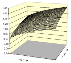
Map of Cobb-Douglas Utility function Click for larger image

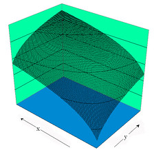
Linear Expenditure Utility function Click for larger image

This is unsatisfying because the result is that there is no feedback on demand from price; demand remains unaffected by the satisfaction that a dollar spent on x yields. In real life, an increase in the price of a thing, such as energy or shelter, will cause one to consume not only less of that thing, but ultimately, seek maximization strategies in which one spends less on that thing. Most of the famous exceptions to this aren't exceptions at all; they involve an increase in income (I).


An alternative to the Cobb-Douglas Utility function is the linear expenditure function. This modifies the utility function to
U(x,y)= α ln (x - x₀) + β ln (y - y₀)
where x₀ and y₀ are given constants, and α + β = 1.

In this case, the optimal values of x*, y* are

p₁x = αI + βp₁x₀ — αp₂y₀
p₂y = βI — βp₁x₀ + αp₂y₀
which can be contrived to alter the shape of indifference curves; say, if we wanted to discuss fuel versus everything else, and then changed the subject to another type of good that is a superior good.