A Digression on Returns to Factor

It is not necessarily so that the income that goes to a factor of production—e.g., labor—is proportionate to that factor's contribution to productivity. First, let's consider the extreme case of a monopoly.

Click image to enlarge The shaded rust-colored area represents the rents captured by the monopolist from the consumer

This is an extreme case, but the difference between the extreme of a monopoly and more common cases of oligopoly (such as price leadership) is not immense. Notice the demand curve for the product is the same as the demand curve for the firm. The curved red line is the marginal cost (MC) curve. The dashed blue line is the marginal revenue (MR) curve; it represents the additional revenue brought in by increasing sales by one more unit.

A few parenthetical notes about the chart: first, I started out with the simplest scenario, in which demand is a linear function of price. In real life, most products have a somewhat concave curve. Second, the point where MC is lowest is chosen arbitrarily. MC may conceivably be downward sloping for the entire range of the graph. For nontrivial examples of a monopoly, though, there's usually a tendency for MC to be rising because of the cost of administration. The shaded represents surplus captured from the consumer by the monopolist (explained). It's the reason classical economists are opposed to monopolies: not because they resent the transfer of wealth, although that's a problem, but the dead weight loss of reduced production and higher costs for all.

Now, let's look at a diagram illustrating factor markets:Here, labor demand is convex because the same firm is facing a production function in which capital can be substituted for labor. When prices are high, then not only are customers restricted by budget, they have the option of replacing labor with equipment. Likewise, the supply curve is usually understood to become much less elastic as wages rise. Put another way, as wages and hours rise, leisure becomes more valuable to workers as well. Of course, these things are dependent on many things, such as the demand curves for many products, the exposure to foreign markets, and so on. But here, we're using the simple assumption that the demand curves for products are straight & diagonal, and that it's not difficult for managers to substitute capital for labor.

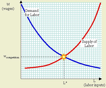
Now, what happens to the demand for labor in a monosonoid firm?

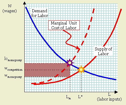
The shaded rust-colored area represents producer surplus captured by the monopsonist from the employee. Note that labor demand for the firm is determined (as before) by the firm's production function, which reflects demand for its products.

Here, there's only one firm with a demand for a specialized type of labor; the most familiar real-life examples are regions. Since the monopsonoid's market dominance is felt in the input market, we would expect to see a deflection from the supply curve. The monopsonoid firm experiences a supply that represents the entire factor market, so when it increases its number of workers, it experiences an increase in marginal wages. This will affect its optimal hiring decision. Hence, it will consider its marginal unit labor cost, which is "inside of" the labor supply curve. It will hire based on the intersection of its internal "demand" for labor (blue line) and the marginal unit labor cost curve. As always, the supply curve will determine wage costs.

The logical extreme is the monopoloid-monopsonoid firm. Again, such an entity is not likely to be seen its pure form, but would illustrate the intermediate-and-plausible case of the oligoloid-oligopsonoid (or segmented) firm, in a market with few participant firms. Here, the concave violet curve reflects the marginal product of labor. For the same reason that the demand for labor was convex, the marginal product declines slowly at first because small amounts of labor can supplement, or replace, a large amount of capital. As L grows, though, the downward slope of the solid violet line reflects the downward slope of the blue demand curve for the product being produced. Moreover, the marginal productivity of labor declines as the amount increases.

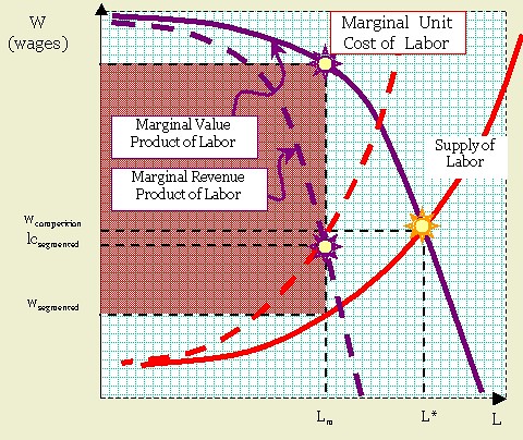
The rust-colored area now includes surplus captured from both consumers (above the point lc_segmented) and from the workers (below).

Reflecting the same rationale as the monopoloid firm, we see how the marginal revenue product declines faster yet. Hence, wages are still determined by the solid labor supply curve, but the firm will prefer to cut off further hiring when labor costs lc reach the level lc_segmented. Above the point lc_segmented, the surplus captured is consumer surplus.

Again, while it is true that a genuine double-m firm is rare, and applies to cases like company towns or haciendas, it's not drastically different from the condition in which a market is dominated by a few large firms. As we can see, there will be significant underemployment of labor, which means that employees will be cherry-picked for productivity, and yet this same underemployment (with its high marginal productivity for labor) will mean a low share of GDP for labor as well. Another point to remember is that this applies to other factors as well; for example, materials (especially from former colonies) and energy inputs.